Introduction

I live in Orlando Florida, which is less than an hour away from Cape Canaveral. As you might imagine, visiting the space center and watching launches is a “thing” we Orlando folks do fairly often.

⊕Me. A long time ago. Pretending to be too close to a launch by posing in front of a photo framed at the Kennedy Space Center. Meta.

I’ve also been getting into R and data science recently via Garrett Grolemund and Hadley Wickham’s excellent R for Data Science. To apply the things I’m learning, I thought it’d be fun to analyze this week’s Tidy Tuesday astronauts dataset.

I’ll follow the analysis process suggested by R for Data Science:

1. Import/Tidy
2. Explore (via Transforming, Visualizing, and Modeling the data)
3. Repeat exploration loop.
4. Communicate results.

If you’re not interested in the journey, you can skip to the results. The graphs are cleaner and there’s no code to clutter things.

Load and Tidy

tuesdata <- tidytuesdayR::tt_load('2020-07-14')

## 
##  Downloading file 1 of 1: `astronauts.csv`

Let’s glimpse our data:

astronauts <- tuesdata$astronauts 
glimpse(astronauts)

## Rows: 1,277
## Columns: 24
## $ id                       <dbl> 1, 2, 3, 4, 5, 6, 7, 8, 9, 10, 11, 12, 13, 14, 15, 16, 17, 18, 19, 20, 21, 22, 23, 24, 25, 26, 27, 28, 29, 30, 3…
## $ number                   <dbl> 1, 2, 3, 3, 4, 5, 5, 6, 6, 7, 7, 7, 8, 8, 9, 9, 9, 10, 11, 11, 12, 13, 14, 15, 15, 16, 17, 17, 17, 17, 17, 17, 1…
## $ nationwide_number        <dbl> 1, 2, 1, 1, 2, 2, 2, 4, 4, 3, 3, 3, 4, 4, 5, 5, 5, 6, 7, 7, 8, 9, 10, 11, 11, 5, 6, 6, 6, 6, 6, 6, 7, 7, 8, 9, 9…
## $ name                     <chr> "Gagarin, Yuri", "Titov, Gherman", "Glenn, John H., Jr.", "Glenn, John H., Jr.", "Carpenter, M. Scott", "Nikolay…
## $ original_name            <chr> "ГАГАРИН Юрий Алексеевич", "ТИТОВ Герман Степанович", "Glenn, John H., Jr.", "Glenn, John H., Jr.", "Carpenter, …
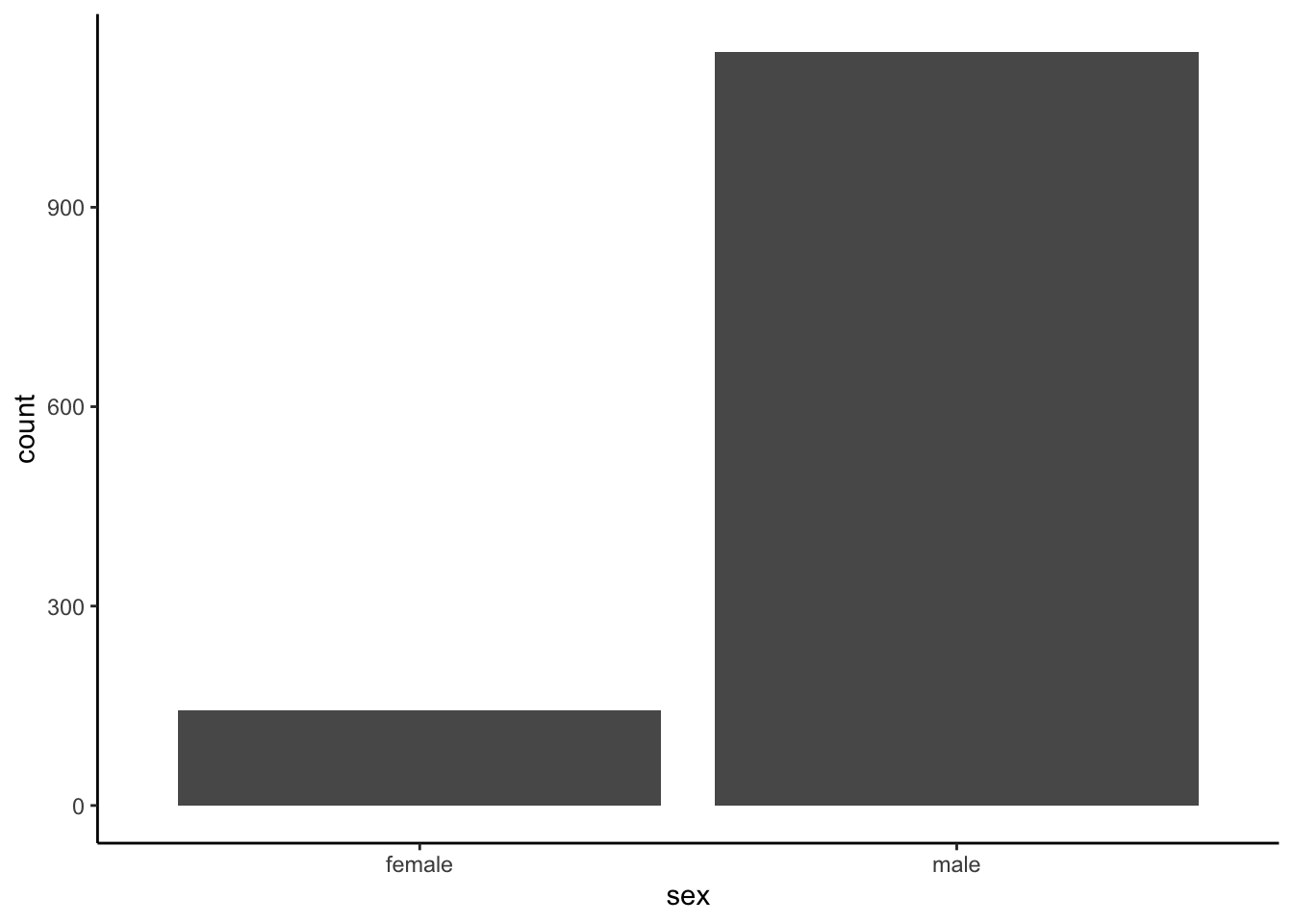
## $ sex                      <chr> "male", "male", "male", "male", "male", "male", "male", "male", "male", "male", "male", "male", "male", "male", …
## $ year_of_birth            <dbl> 1934, 1935, 1921, 1921, 1925, 1929, 1929, 1930, 1930, 1923, 1923, 1923, 1927, 1927, 1934, 1934, 1934, 1937, 1927…
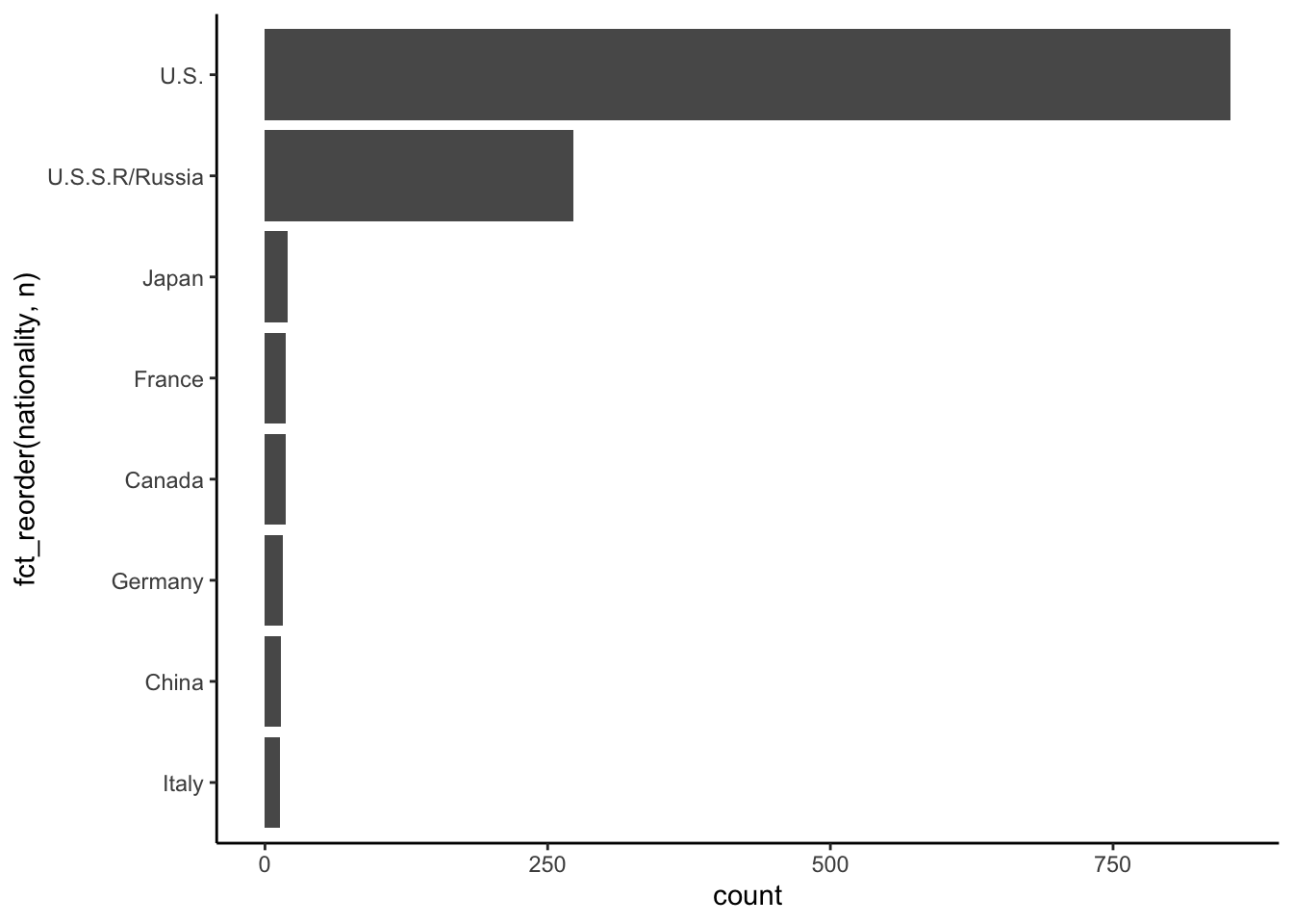
## $ nationality              <chr> "U.S.S.R/Russia", "U.S.S.R/Russia", "U.S.", "U.S.", "U.S.", "U.S.S.R/Russia", "U.S.S.R/Russia", "U.S.S.R/Russia"…
## $ military_civilian        <chr> "military", "military", "military", "military", "military", "military", "military", "military", "military", "mil…
## $ selection                <chr> "TsPK-1", "TsPK-1", "NASA Astronaut Group 1", "NASA Astronaut Group 2", "NASA- 1", "TsPK-1", "TsPK-2", "TsPK-1",…
## $ year_of_selection        <dbl> 1960, 1960, 1959, 1959, 1959, 1960, 1960, 1960, 1960, 1959, 1959, 1959, 1959, 1959, 1960, 1960, 1960, 1962, 1960…
## $ mission_number           <dbl> 1, 1, 1, 2, 1, 1, 2, 1, 2, 1, 2, 3, 1, 2, 1, 2, 3, 1, 1, 2, 1, 1, 1, 1, 2, 1, 1, 2, 3, 4, 5, 6, 1, 2, 1, 1, 2, 3…
## $ total_number_of_missions <dbl> 1, 1, 2, 2, 1, 2, 2, 2, 2, 3, 3, 3, 2, 2, 3, 3, 3, 1, 2, 2, 1, 1, 1, 2, 2, 1, 6, 6, 6, 6, 6, 6, 2, 2, 1, 4, 4, 4…
## $ occupation               <chr> "pilot", "pilot", "pilot", "PSP", "Pilot", "pilot", "pilot", "pilot", "commander", "pilot", "commander", "comman…
## $ year_of_mission          <dbl> 1961, 1961, 1962, 1998, 1962, 1962, 1970, 1962, 1974, 1962, 1965, 1968, 1963, 1965, 1963, 1976, 1978, 1963, 1964…
## $ mission_title            <chr> "Vostok 1", "Vostok 2", "MA-6", "STS-95", "Mercury-Atlas 7", "Vostok 3", "Soyuz 9", "Vostok 4", "Soyuz 14", "Mer…
## $ ascend_shuttle           <chr> "Vostok 1", "Vostok 2", "MA-6", "STS-95", "Mercury-Atlas 7", "Vostok 3", "Soyuz 9", "Vostok 4", "Soyuz 14", "Mer…
## $ in_orbit                 <chr> "Vostok 2", "Vostok 2", "MA-6", "STS-95", "Mercury-Atlas 7", "Vostok 3", "Soyuz 9", "Vostok 4", "Soyuz 14", "Mer…
## $ descend_shuttle          <chr> "Vostok 3", "Vostok 2", "MA-6", "STS-95", "Mercury-Atlas 7", "Vostok 3", "Soyuz 9", "Vostok 4", "Soyuz 14", "Mer…
## $ hours_mission            <dbl> 1.77, 25.00, 5.00, 213.00, 5.00, 94.00, 424.00, 70.93, 377.00, 9.22, 25.87, 260.13, 34.32, 191.92, 119.13, 189.0…
## $ total_hrs_sum            <dbl> 1.77, 25.30, 218.00, 218.00, 5.00, 519.33, 519.33, 448.45, 448.45, 295.20, 295.20, 295.20, 225.00, 225.00, 497.8…
## $ field21                  <dbl> 0, 0, 0, 0, 0, 0, 0, 0, 0, 0, 0, 0, 0, 0, 0, 0, 0, 0, 0, 0, 0, 0, 0, 1, 0, 0, 0, 0, 0, 3, 0, 0, 0, 0, 1, 0, 0, 2…
## $ eva_hrs_mission          <dbl> 0.00, 0.00, 0.00, 0.00, 0.00, 0.00, 0.00, 0.00, 0.00, 0.00, 0.00, 0.00, 0.00, 0.00, 0.00, 0.00, 0.00, 0.00, 0.00…
## $ total_eva_hrs            <dbl> 0.00, 0.00, 0.00, 0.00, 0.00, 0.00, 0.00, 0.00, 0.00, 0.00, 0.00, 0.00, 0.00, 0.00, 0.00, 0.00, 0.00, 0.00, 0.00…

Each row is an astronaut and the mission they accomplished. Columns are variables whose meaning is fairly clear from the name, with the exception of field21.

Let’s rename it. The docs say that it represents “Instances of EVA by mission.”:

astronauts <- astronauts %>% 
  rename(evas_by_mission = field21)

Exploration Loop 1

I’m curious what the spread of astronauts is by sex.

astronauts %>% 
  ggplot(aes(sex)) +
  geom_bar()

Unfortunately, this isn’t surprising. I wonder if the ratio of male to female astronauts has become more equal over time.11 I’m going to have a daughter soon, and if she wants to be an astronaut, I sure hope she doesn’t have to deal with any bias. Let’s see:

astronauts %>%
  ggplot(aes(year_of_mission, fill = sex)) +
  geom_bar()

It’s not crystal clear from here whether the ratio has improved over time. Let’s confirm explicitly by creating, plotting, and fitting a line to a ratio variable.

astronauts %>%
  group_by(year_of_mission) %>% 
  summarise(ratio = sum(sex == "female") / sum(sex == "male")) %>% 
  ggplot(aes(year_of_mission, ratio)) +
  geom_point() + 
  geom_smooth(se = F)

## `summarise()` ungrouping output (override with `.groups` argument)

## `geom_smooth()` using method = 'loess' and formula 'y ~ x'

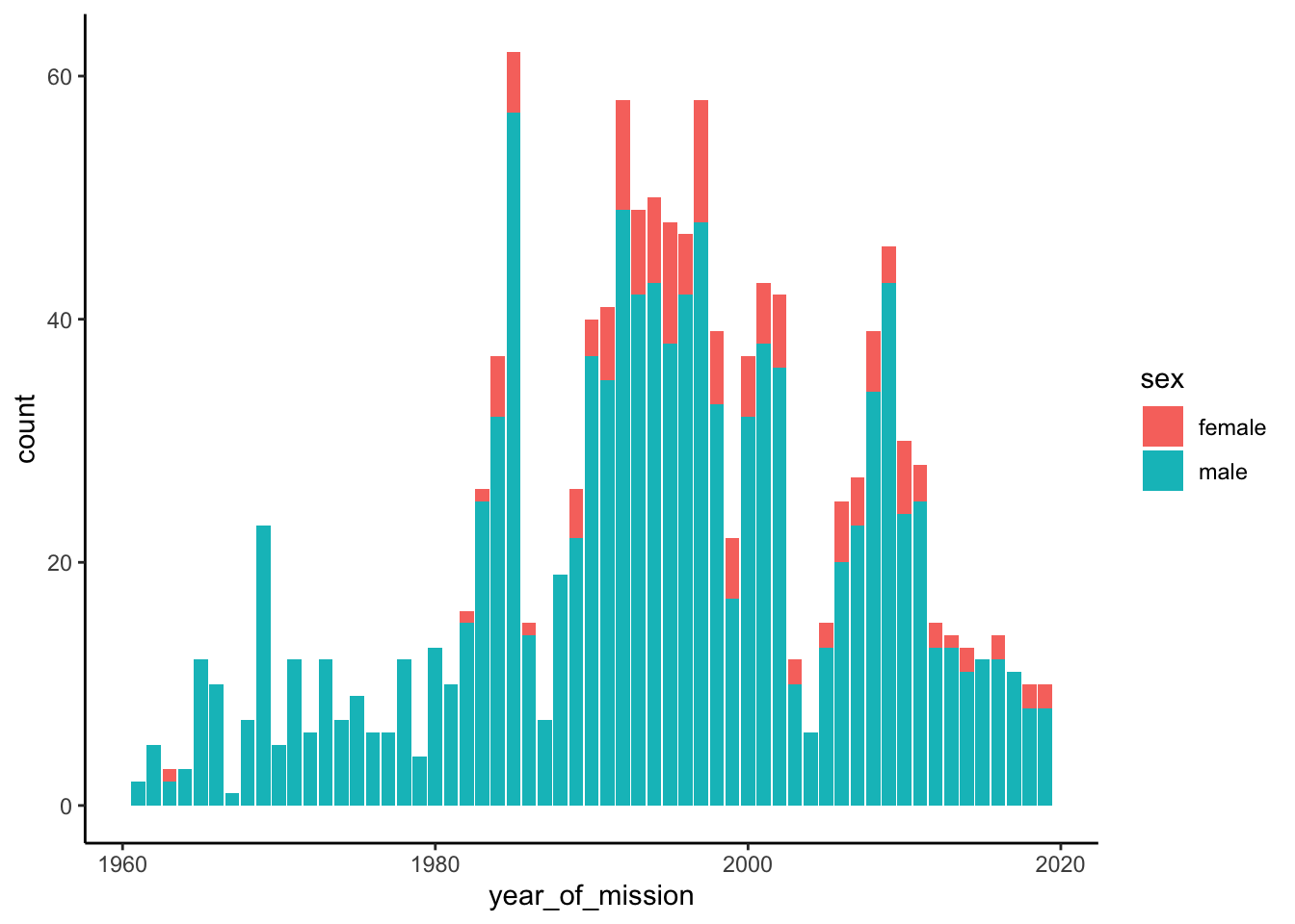
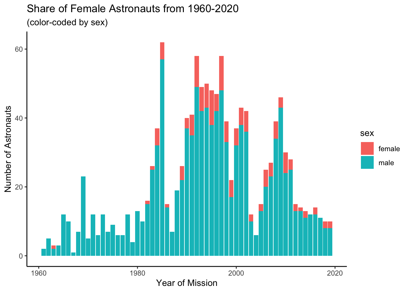
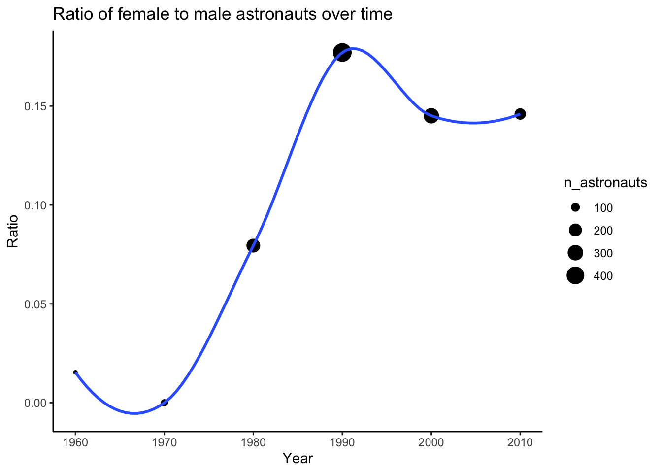
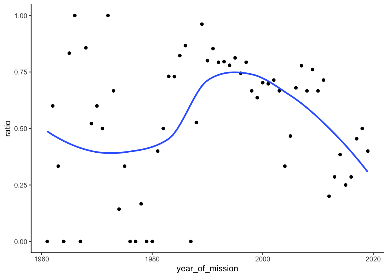
Looks like there was more equality since the 60s, but there may be some tapering off starting in the 2000s.

What the heck happened in ~1960? That’s an unusually high ratio.

astronauts %>% 
  filter(between(year_of_mission, 1960, 1970)) %>% 
  group_by(year_of_mission) %>% 
  count(sex)

## # A tibble: 11 x 3
## # Groups:   year_of_mission [10]
##    year_of_mission sex        n
##              <dbl> <chr>  <int>
##  1            1961 male       2
##  2            1962 male       5
##  3            1963 female     1
##  4            1963 male       2
##  5            1964 male       3
##  6            1965 male      12
##  7            1966 male      10
##  8            1967 male       1
##  9            1968 male       7
## 10            1969 male      23
## 11            1970 male       5

Ah. Only three astronauts went on missions in 1963 and one of them was female. Makes sense now.

Exploration Loop 2

I’m curious what the spread of astronauts is by nationality.

astronauts %>% 
  ggplot(aes(nationality)) +
  geom_bar()

That’s not useful. Let’s drop nationalities that appear less than 10 times in the dataset, flip the axis, and sort.

astronauts %>% 
  add_count(nationality) %>% 
  filter(n > 10) %>% 
  ggplot(aes(x = fct_reorder(nationality, n))) +
  geom_bar() +
  coord_flip()

Better. Looks like the US dominates missions overall.

Let’s try looking at the the ratio of US astronauts on missions over time:

astronauts %>%
  group_by(year_of_mission) %>% 
  summarise(ratio = sum(nationality == "U.S.") / n()) %>% 
  ggplot(aes(year_of_mission, ratio)) +
  geom_point() + 
  geom_smooth(se = F)

## `summarise()` ungrouping output (override with `.groups` argument)

## `geom_smooth()` using method = 'loess' and formula 'y ~ x'

Interesting. I didn’t realize the U.S. peaked in terms of share of astronauts sent to space in the mid-90s. This makes me wonder how the number of U.S. missions have changed over time.

astronauts %>% 
  count(year_of_mission, wt = sum(nationality == "U.S.")) %>% 
  ggplot(aes(year_of_mission, n)) +
  geom_point() + 
  geom_smooth(se = F)

## `geom_smooth()` using method = 'loess' and formula 'y ~ x'

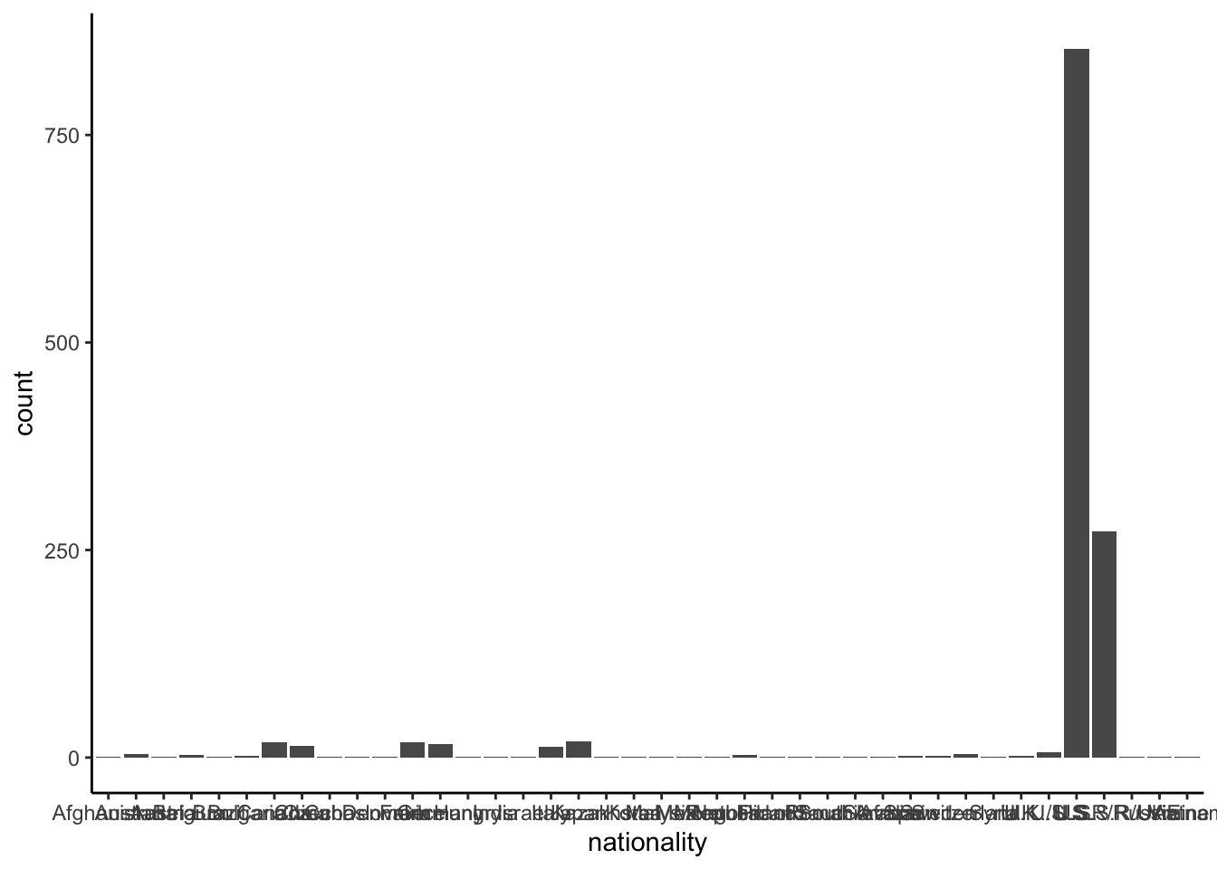
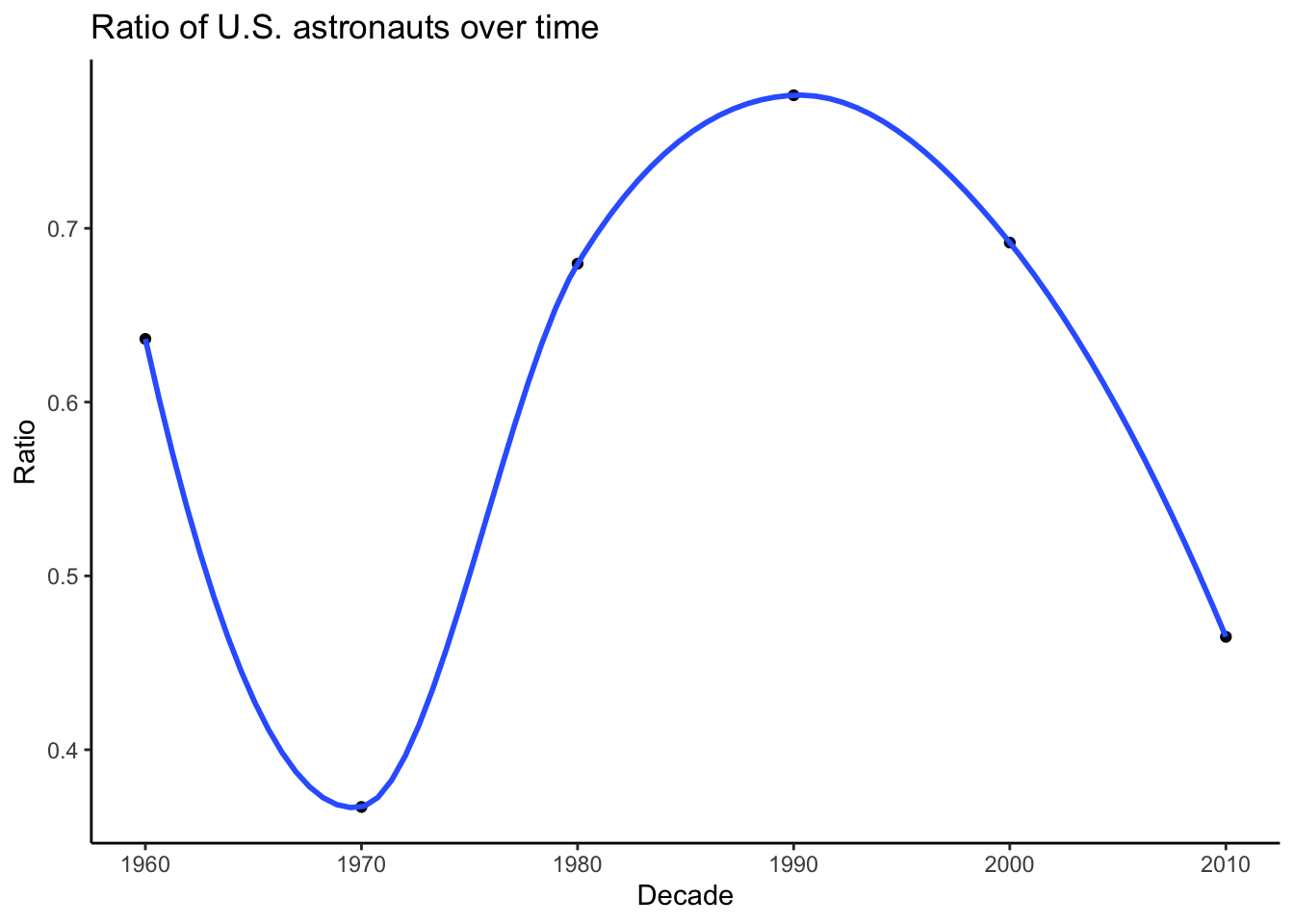
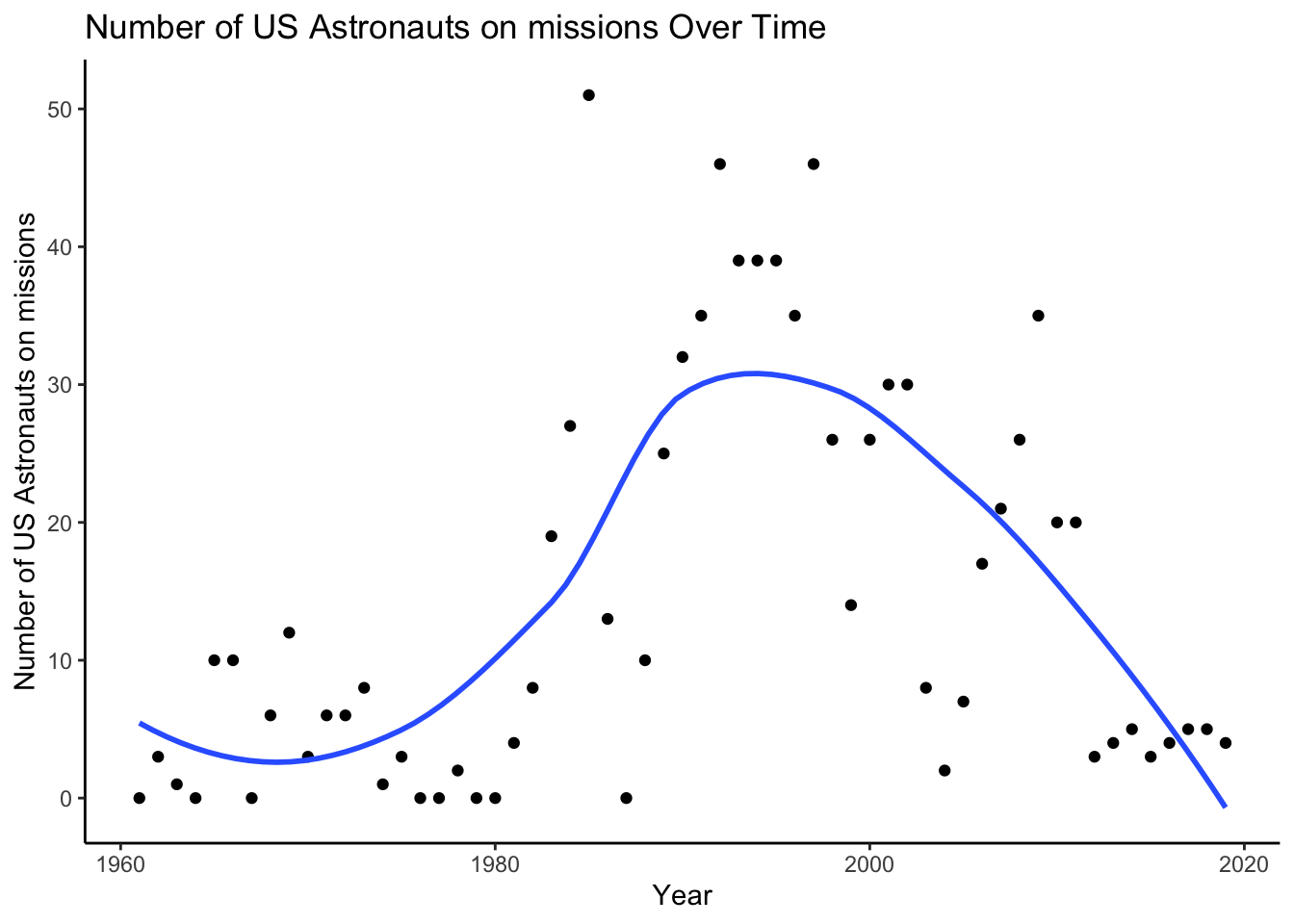
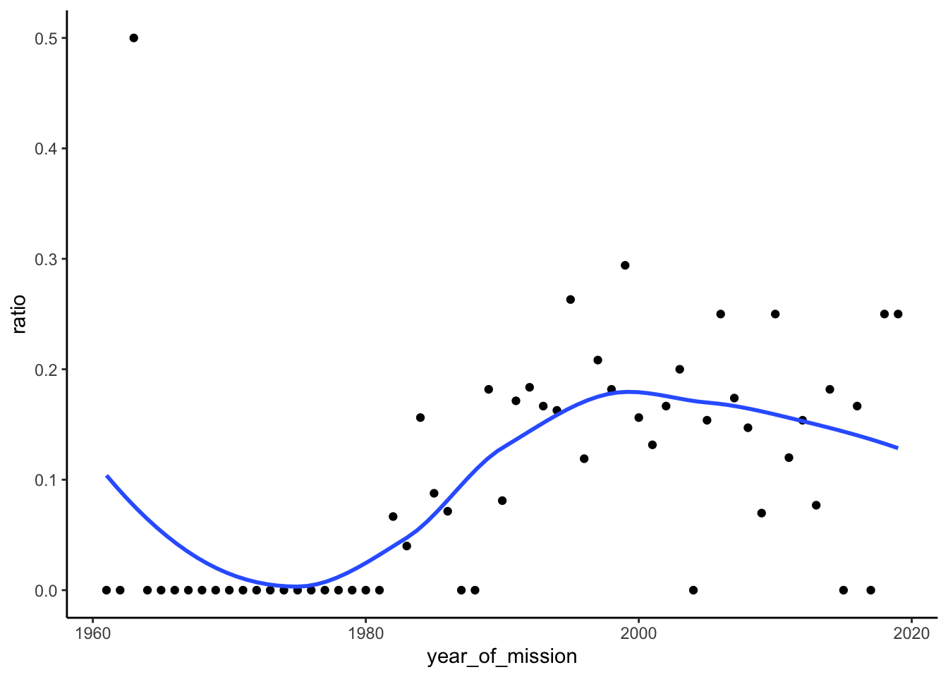
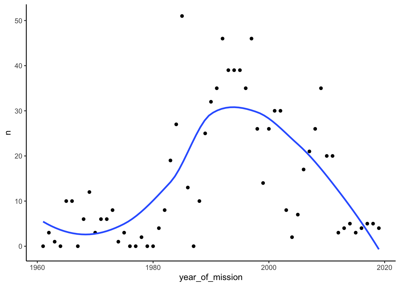Super interesting! I remember thinking that Obama’s shutting of the shuttle program would be an inflection point of NASA’s activity, but this suggests that the inflection point was before Obama was even elected: ~1994.

Results

This data set suggests three interesting conclusions: